Introduction to Radio Interferometry

Introduction to my Blog

Hello and welcome to my blog! As this is my first post, I thought I’d quickly introduce myself before we delve into my introduction to interferometry. My name is Devin and I’m currently a graduate student at Caltech studying towards a master’s degree in Electrical Engineering. My primary interest is instrumentation. My passion is building hardware systems that allow us to better understand the world around us (e.g. radio telescopes, quantum circuits, sounding rockets). However, a lot of the work that I’ve done has been bringing these types of systems to life through software development, so I consider myself a bit of a mixed bag of skills and expertise. If you’re interested in learning more about what I do or how I do it, please check out my website here.

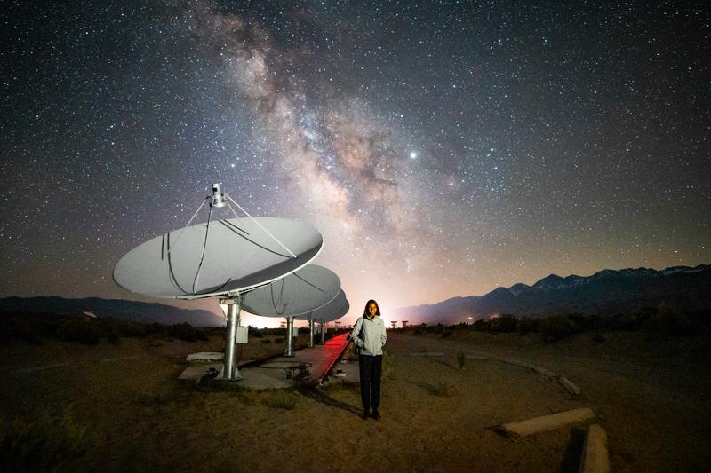
At Caltech, I’m working with Gregg Hallinan and Sandy Weinreb on a project called the OVRO Long Wavelength Array (LWA). The LWA is a radio interferometer composed of 256 discrete dipole antennas that produces images of the radio sky every 10 seconds. This project is particularly exciting for me because I’ve always been interested in how many distinct dishes can synthesize coherent images, sometimes with resolutions that cannot be achieved with single dish telescopes.

Radio interferometry often comes off as a difficult concept, but it doesn’t need to be that way. In this blog post, I will attempt to give a more intuitive introduction to radio interferometry, one that, in particular, might help a budding radio engineer learn more about this fascinating field. I will assume knowledge of calculus, but everything else will be developed from the ground up.

So What are Radio Interferometers?

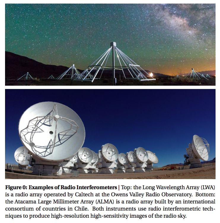
By way of introduction to the topic of interferometry, I thought I’d show images of two radio interferometers (see fig. 0). Radio Interferometry is a method by which many distinct dishes (such as ALMA) or many distinct dipoles (such as the LWA) are used together to produce images of the radio sky. Although the earliest radio telescopes used single dishes, the majority of radio telescopes being built today are interferometers. This is because interferometers are generally able to produce higher-resolution and higher-sensitivity images than their single dish counter-parts.

Starting with the Punchline

My plan is to start with the big punchline of radio interferometry and then work backwards to then justify everything else. So, are you ready for it? The big reveal? Ok, here it is: the most mind-blowing fact about radio astronomy is that instead of directly observing the sky, radio interferometers measure the Fourier transform of the sky. Slow down, don’t leave just yet, let’s take a minute to break this down. The Fourier transform is a method of taking a sequence of data which is represented in one way (i.e. a series of measurements over time, a signal coming from a sensor, or series of pixels across a spatial grid¹) and representing it in a different, but equally valid way. When you take the Fourier transform of some data, no information is lost. The data has simply been rearranged. Simultaneously, there exists a method by which we can take some data which has been Fourier transformed and undo the Fourier transform to recover the original data. This procedure is called the inverse Fourier transform. The important thing to take away from this, is that if we measure the Fourier transform of the sky with an interferometer, then we can reconstruct an map (image) of the sky brightness by taking the inverse Fourier transform of that data. But enough words, let’s look at some pictures.

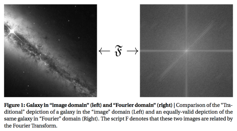
Fig. 1 shows two entirely equivalent, equally valid representations of a galaxy. The image on the left is an image you might find in an Astronomy 101 textbook and the image on the right is simply the Fourier transform of the image on the left². It is just as true, however, to say that the image on the left is the inverse Fourier transform of the image on the right.

Radio interferometry is a method of collecting information about the sky in the “Fourier” domain (i.e. information similar to that shown on the right in Fig. 1). Once we have collected this information, we can then use a computer to compute the inverse Fourier transform of the data and thereby reconstruct a picture of the sky.

But how does an interferometer measure the Fourier transform of the sky? To answer this question, we will start by examining how the one-dimensional Fourier transform works.

The (Discrete) Fourier Transform

At its core, the one-dimensional (Discrete³) Fourier transform states that any signal, that is, any sequence of N data points (e.g. measurements of position, a stock’s value over time, or pixel intensities in a one-dimensional image) with regular spacing can be represented by (decomposed into) a sum of N/2+1 sines and N/2+1 cosines.

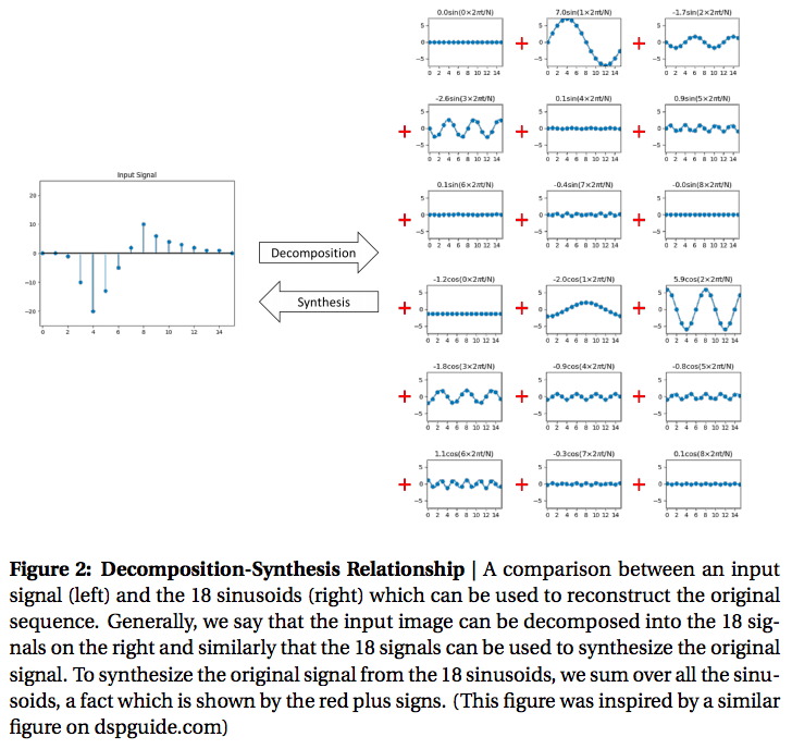
Fig 2. shows an example of this relationship with a signal⁴ of length 16. On the left side of Fig 2. we show a 16-point signal which has been decomposed into (16/2+1 =) 9 sine and 9 cosine waves as shown on the right. Equivalently, we can say that the 18 signals on the right can be synthesized (summed) to form the signal on the left. These two representations are exactly equivalent in the information that they contain. As Steven Smith, author of “The Scientist and Engineer’s Guide to Digital Signal Processing”, points out, “There is no difference between the [original signal] and the sum of the signals in [the decomposition], just as there is no difference between 7 and 3+4”.

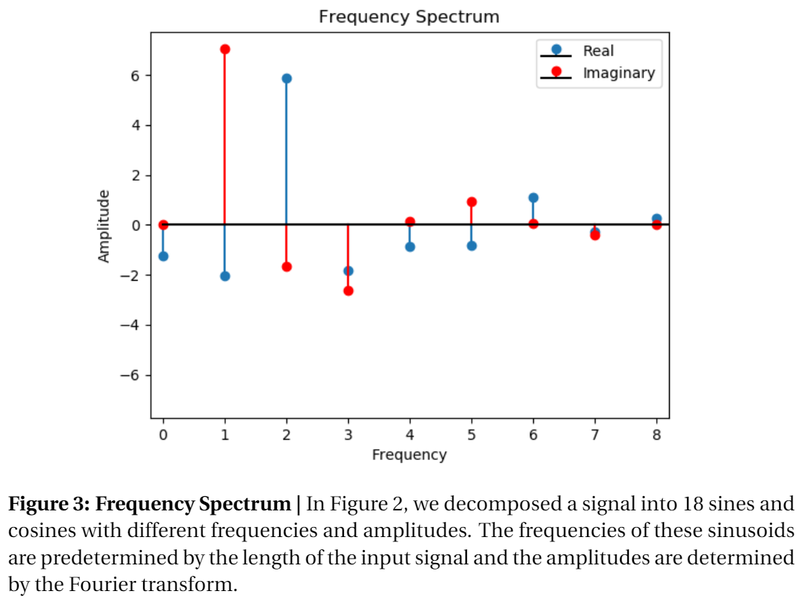
Often times, it’s more useful to represent the information about the Fourier decomposition as a frequency spectrum. Fig. 3 shows the frequency spectrum of the signal in Fig. 2. In this plot, the amplitudes of the sinusoids are plotted as functions of their frequencies. Notice that all the important information is contained within this plot. As you will remember from trigonometry, a sinusoid is completely determined by its frequency (X-axis), amplitude (Y-axis), and phase (sine corresponds to the real part, while cosine corresponds to the imaginary part). The actual values which comprise each sinusoid are omitted since they can be uniquely determined from the frequency, amplitude, and phase. Typically, when someone asks for the Fourier Transform of a signal, this is the information they are looking for.

The Fourier transform determines how much of each sinusoid is needed by using a technique called correlation. At its core, correlation is a method which allows us to determine how much “sameness” is contained in the two signals.

Mathematically, correlation is about as fundamental an operation as they come, and in-fact, you might already know about it by its other name: the dot product. Simply multiply each element in the two sequences (signals) and add all the products together. In geometric terms, correlation can also be thought of as the projection of one signal onto the other. The Fourier transform finds the amplitudes of all of the necessary sines and cosines by finding the “sameness” between the input signal and “test sinusoids” – signals with predetermined frequencies and unit amplitudes.

Let’s see what this looks like mathematically. The equation for correlation between two signals, \( x[n] \) and \( y[n] \) is

$$ x\cdot y = \sum_{n=1}^{N-1}x[n]y[n] $$

All this equation is doing is multiplying each term in the two sequences and adding up the result. The Fourier transform is simply an extension of this equation. Lets look at the equation for the Fourier transform⁵

$$\mathfrak{Re}\{X[k]\} = \frac{2}{N}\sum_{n=1}^{N-1}x[n]\cos(2\pi kn/N)$$

$$\mathfrak{Im}\{X[k]\} = \frac{2}{N}\sum_{n=1}^{N-1}x[n]\sin(2\pi kn/N)$$

where

$$ k \in \mathbb{Z} \cap [0, N/2 ] $$

These equations might look scary, but let’s work through them together. Here \( x[n] \) (note that little \( x[n] \) and big \(X[k]\) are different even though they are representations of the same signal) is the signal that we are analyzing, and \( y[n] \) has been replaced by \(\cos(2\pi kn/N)\). This is simply our test sinusoid. The frequency of each test sinusoid is set by the parameter k and the third equation \( (k \in \mathbb{Z} \cap [0, N/2 ]) \) tells us that the frequency takes integer values between \(0\) to \(N/2\) inclusive. \(X[k]\) is the variable that will hold the amplitudes of our decomposed signal. Evidently, the real part of \(X\) will hold the amplitudes of the cosines and the imaginary part of \(X\) will hold the amplitudes of the sines. Using exact nomenclature, \(X[k]\) is the representation of \( x[n] \) in the Fourier domain. Finally, the Fourier transform scales each of these correlations by \(2/N\) to set the appropriate scale when things are added together again.

In a similar manner, given \(X[k]\), we can use the inverse Fourier transform to synthesize \( x[n] \):

Here, we are using the amplitudes stored in \(X[k]\) to scale the 18 sinusoids and sum them together. Notice that the amplitudes derived in the Fourier tranfrom become the amplitudes for the same test sinusoids in the inverse transform. That is to say, if \( \mathfrak{Re}\{X[2]\} \) is the amplitude which corresponds to the result of the correlation between the input and the test sinusoid \(\cos(4\pi n/N)\) during the Fourier transform, then \( \mathfrak{Re}\{X[2]\} \)will be the amplitude of the \(\cos(4\pi n/N)\) term during the inverse Fourier Transform.

Let’s now take a deeper look at the mechanics of correlation as used in the Fourier transform. Fig. 4 shows what this might look like graphically.

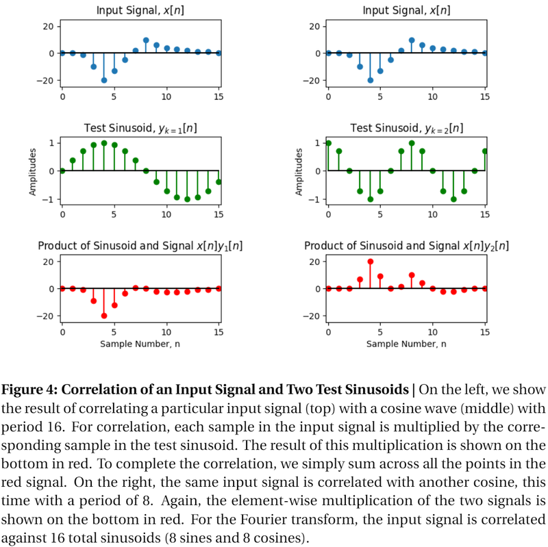
Fig. 4 shows the correlation of one input signal with two different test sinusoids. The test sinusoid on the left is a sine wave with frequency \(k = 1\) and amplitude 1 while the one on the right is a cosine with frequency \(k = 2\) and amplitude 1. As described in the correlation equation, we multiply all of the values in our sequence, \(x\), \((x[1], x[2], \cdots x[n]) \) with their corresponding values in the test sinusoid \( (y[1], y[2], \cdots y[n]) \) . The result of this multiplication is shown on the bottom for both of these test sinusoids. To complete the correlation, we sum all of the products together which gives us a single scalar value. Once we have done the above operation for a sine and cosine at each frequency, we will have all the information to write down the Fourier transform of the signal.

Correlation on the Sky: Putting it All Together

Now that we’ve gotten a better understanding of the Fourier transform, We now have the tool we need to calculate the amplitudes of the sinusoids which exactly decompose our original signal. To recap, we simply correlate our original signal with a toolbox of test sinusoids (one sine and one cosine at each of the N/2+1 frequencies and then we can represent our signal as a sum of those same test sinusoids with a new amplitude.

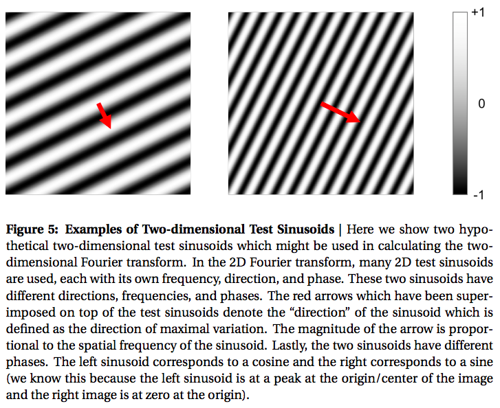
For the two-dimensional Fourier transform, we do the exact same thing, except this time, our test sinusoids look like the one shown in Fig. 5. Furthermore, we have to sum over two-dimensions (one for the x direction and one for the y direction). For the two-dimensional Fourier transform, the “direction” of the sinusoid (that is, the direction of maximal variation) varies by 360 degrees, in Fig. 5 we show two possible frequencies and directions which are denoted by the red arrows.

Now, let’s return to radio astronomy and attempt to answer the question that spurred this adventure into the Fourier transform in the first place: how does an interferometer measure the Fourier transform of the sky? The answer, of course, is with test sinusoids! Supposing we had an “instrument” with an antenna pattern (also known as a beam pattern or radiation pattern) that looked like the sinusoid shown in Fig. 5, then by observing the sky with this instrument, the signal coming from the antenna would be the Fourier amplitude needed for the Fourier decomposition. Remember that an antenna pattern tells us the directional dependence of the antenna’s sensitivity to radiation.

Let’s examine what happens visually to images when they are “measured” by a beam pattern. Ultimately, we will see that this measurement looks a lot like a two-dimensional correlation. Suppose we have a “radiation intensity distribution” on the sky which looks like the galaxy in Fig. 1 where the white parts of the image correspond to high intensity radiation and black corresponds to no radiation from that direction. To calculate the amount of power received by the antenna, we multiply the intensity of the distribution in every direction by the ability of the antenna to receive power from that direction (i.e. the beam pattern) and sum over all these directions. Mathematically,

Where \(x[i,j]\) is our intensity distribution and \(y[i,j]\) is our beam pattern. This is precisely the formulation for a two-dimensional correlation. Note that in these examples, we are correlating on a cartesian grid, however, in general, the beam patterns and intensity distributions are defined on spherical grids. (see here or here for review on beam patterns).

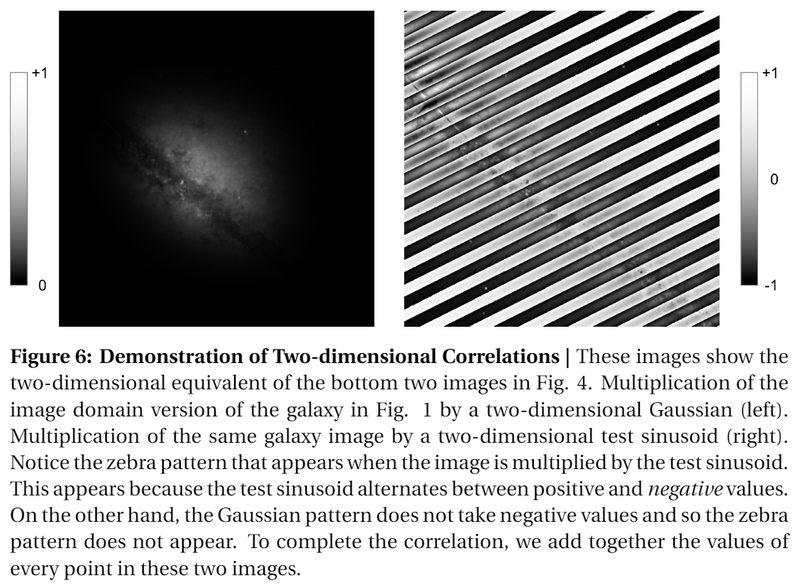
Fig. 6 shows the intermediary result after multiplication but before summation for two beam patterns. In effect, the images in Fig. 6 show the intensity of the recieved radiated power from any directions. For example, when measured by an antenna with a gaussian beam pattern, the instument receives more power from the center of the image than the the edges. When measured by (correlated with) a test sinusoid, a distinctive zebra pattern arises because the test sinusoid alternates between both positive and negative values.

Last, and most importantly, if we had many instruments each with a different test sinusoid beam pattern, then we’d be able to calculate the Fourier amplitudes for all of these sinusoids and exactly determine how the sky is represented in the Fourier domain⁶.

The Fringe Pattern

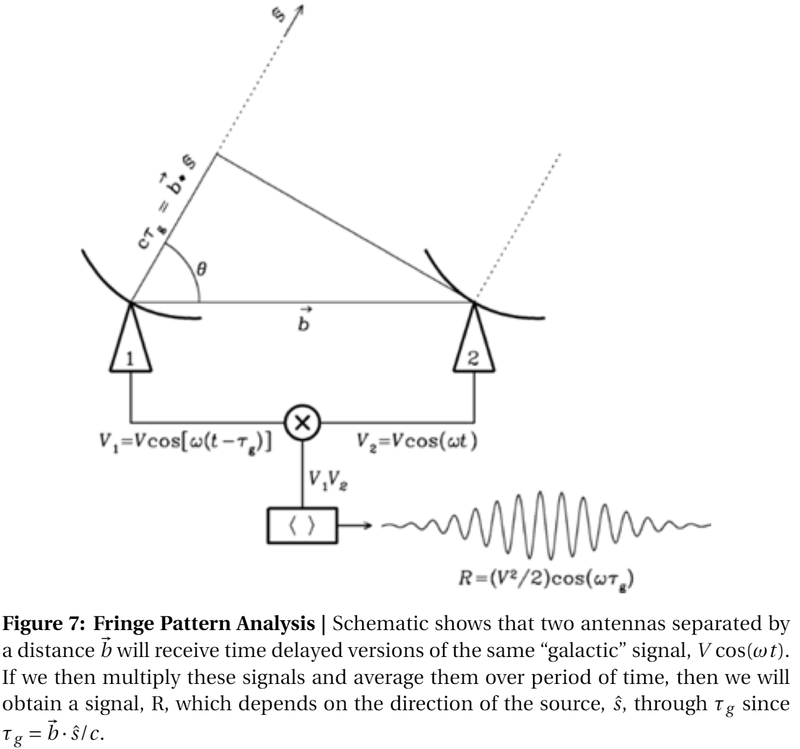
Finally, we will now turn to Fig. 7, which is commonly the first image shown during lectures on Interferometry. Fig. 7 is fundamentally a blueprint for the design of an instrument which has beam pattern that approximates a test sinusoid.

The derivation proceeds as follows: suppose we have two antennas, separated by some vector b looking at some object in the sky in the direction given by the unit vector, \(\hat{s}\). Assuming that the object (source) in the direction of \(\hat{s}\) is far enough away that the radiation from it can be assumed to be a plane wave⁷, then the time delay between when radio telescope number 2 receives the signal and when radio telescope number one receives the signal is given by \(\tau_g\). \(\tau_g\) is calculated by the equation

$$c\tau_g = \vec{b} \cdot \vec{s} = |\vec{b}|\cos(\theta)$$

Thus, if antenna 2 produces some waveform⁸ due to the radiation from \(\hat{s}\), given by

$$V_2(t) = V\cos(\omega t)$$

Then antenna 1 produces some time-delayed version of the same waveform

$$V_1(t) = V\cos(\omega (t-\tau_g))$$

As per Fig. 7, we next multiply these signals together

$$V_{12}(t) = V_1(t)V_2(t) = V^2\cos(\omega t)\cos(\omega (t-\tau_g)$$

Applying a handy trigonometric product identity,

$$V_{12}(t) = \frac{V^2}{2}\cos(\omega \tau_g) + \cos(\omega (2t-\tau_g)).$$

Finally, we average this signal over a long enough period of time such that the temporally varying portion of the signal, \(\cos(\omega(2t-\tau_g))\), averages to 0 and we are left with the following signal, R, which is a function of \(\tau_g\):

Re-writing this in terms of theta, we find that:

$$R(\theta) = \frac{V^2}{2}\cos(\omega |\vec{b}|\cos(\theta)/c)$$

This, at long-last, is our test sinusoid (in proper radio astronomy nomenclature, this pattern is closely related to the interferometer fringe pattern⁹). Fig. 8 plots the above equation for R as we sweep theta from one side of the sky to the other (left). The instrument is most sensitive in the directions of the sinusoidal maxima and has “negative” sensitivity at the locations of the dips.

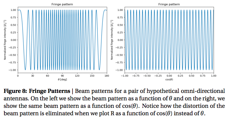
But, wait, you might say, Fig. 8 doesn’t look like the two-dimensional pattern shown in Fig. 5! And you’d be right, they do not look the same; for starters, Fig. 8 is a one-dimensional pattern, and second, Fig. 8 is not a pure cosinusoidal pattern. The answer to the first observation is that the equation for the test sinusoid, R, actually is a 2-dimensional pattern, we simply choose to only plot R in one-dimension (i.e. in \(\theta\)). If we let \(\phi\) be the 2nd angle of a coordinate system where \(\phi\) is orthogonal to \(\theta\), then we can plot R as a function of \(\theta\) and \(\phi\), then we will indeed find that R looks like a two-dimensional test sinusoid.

We will address the second observation, that R is distorted, using a transformation of variables. First, notice that the only difference between our equation for R and a pure cosine is that R is a function of \(\cos(\theta)\) and not \(\theta\). If we were somehow able to removed the cosine, then we would have an ideal sinusoidal testing pattern. This can be accomplish with the following transformation of variables: instead of considering R as a function of \(\theta\), we define new variables, u and v, given by the relations \(u = \cos(\theta)\) and \(v = \cos(\phi)\). Now our two spatial dimensions are not directly functions of \(\theta\) and \(\phi\), but in their cosines, u and v

$$R(u,v) = \frac{V^2}{2}\cos(\omega |\vec{b}|u/c).$$

As if by magic, our test sinusoid is no longer distorted. Note that we restrict theta and phi to be 0 to +180 degrees (i.e. horizon to horizon) such that the mappings from \(\theta\) to \(\cos(\theta)\) and \(\phi\) to \(\cos(\phi)\) is one-to-one. That is to say there is exactly one value of \(\cos(\theta)\) for every value of \(\theta\) and the same goes for \(\phi\). Practially, what this means is that we are transforming the mapping of the sky to some coordinate system in which our test sinusoids are ideal, then once we’ve collected in the Fourier domain and transfered it back to the image domain, we can re-map this data to an actual map of the sky using the same \(u,v\) relations¹⁰.

Lastly, you may wonder how we can generate all the other test sinusoides. Notice that the spatial frequency (i.e. how rapidly the signal, R, peaks and dips as a function of \(\hat{s}\) of our test sinusoid is dependent on \(\vec{b}\), the length and direction¹¹ of the baseline between the antennas. Therefore, although any given pair of antennas is only able to produce one baseline (assuming the antennas don’t move¹²), we can add additional antennas to produce additional baselines and more test sinusoids¹³. With a sufficient number of antennas, we will be able to complete our map of the sky in the Fourier domain, and then, using a computer, transform that data through the inverse Fourier transform to obtain the intensity sky mappings for which interferometry is so renowned.

Outro

This completes my (hopefully) intuitive approach to interferometry. I hope you enjoy reading this as much as I enjoyed writing it. To maximize simplicity, I inevitably had to cut out many interesting and exciting (some might even say critical) aspects of interferometry. However, those details are recorded in greater depth and eloquence than I could ever hope to achieve in such texts as “Interferometry and Synthesis in Radio Astronomy” by A. Richard Thompson, James M. Moran, and George W. Swenson Jr. and “Essential Radio Astronomy” by James Justin Condon and Scott M. Ransom. I would also highly recommend “The Scientist and Engineer’s Guide to Digital Signal Processing” by Steven Smith, a book that was highly influential on my approach to the Fourier transform.

Please feel free to leave a comment or connect with me about this post or anything else that I’m working on! You can reach me at: devin.cody@gmail.com