An Intuitive Interpretation Of The Fourier Transform (or The Link Between Fourier Analysis And Linear Algebra)

Introduction

I despised the Fourier transform.

I didn’t understand why the mathematics worked the way they did. And I couldn’t fathom how anybody could have just sat down and wrote down the equations. To me, the synthesis and decomposition equations appeared almost magically. No physical interpretation. No explanation of why the mathematics should work the way they did.

Now, the Fourier transform is one of tools that I use most often. It took me a long time to gain a physical intuition for the Fourier transform, but now that I have it, I’ve decided that its too exciting not to share.

My objective with this blog post is not to belabor the mechanics of the Fourier transform or attempt to explain every intricate property of the Fourier transform. Rather, my objective is to show you a way of understanding the Fourier transform from a linear algebraic perspective. Once you gain an appreciation for this connection, many of the subtleties of the Fourier transform become almost obvious when observed through this lens¹.

A word of warning before we start: If you’ve never seen the Fourier transform before, this may not be the best place to start your journey. Fear not, however, you can find a good explanation of the (discrete) Fourier transform in my last blog post although I will probably repeat some of the points that I made there. I also recommend the following learning resources: Steve Smith’s Book and Brian Douglas’ YouTube series. I also quite like the explanation given by betterexplained.com

The Punchline

As with my introduction of interferometry, I’m going to start with the punchline and then work backwards to understand what it means and why it’s important. So here it is: the Fourier transform is a (linear) transformation between the standard orthonormal basis and a second orthonormal basis (the Fourier basis).

Now that we know the punchline, let’s take some time to really understand what we mean by orthonormal bases and transformations.

Basis vectors

An implicit assumption of linear algebra is that each number in a vector has some physical meaning. For example, in the three vector, (1,1,1), the first position might represent a one-unit step in the x-axis, the second position might represent the one-unit step in the y-axis, and the third position might represent the one-unit step in the z-axis. The numbers in the vectors then represent how much of each direction is needed to “build” the vector.

Change of Basis

Note, however, the x, y, and z axes are not always the most convenient axes for expressing the vector. Consider the following vectors:

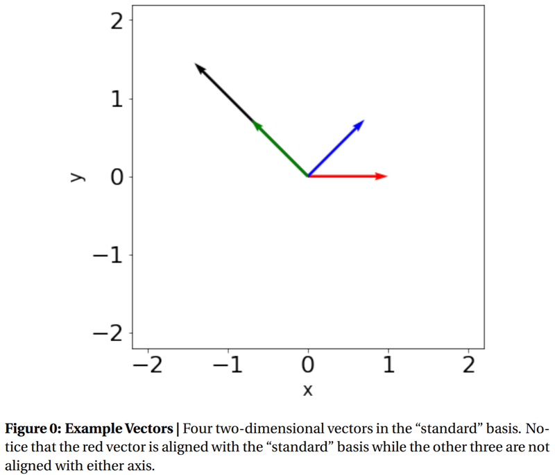
Figure 1: Four two-dimensional vectors in the “standard” basis. Notice that the red vector is aligned with the “standard” basis while the other three are not aligned with either axis.

When written numerically, the vectors take the form (counter-clockwise from red to black):

The first thing to notice here is that the red vector’s representation is simpler than the other vectors’ representations. Although some people may disagree, mathematicians generally prefer simplicity over complexity. When given the option between vectors with many zeros and only a few zeros, it’s preferable to pick the vector with many zeros. For example, the vector \((1,0,0,0)\) is in general better than the vector \( (1,2,3,4)\). In linear algebra, this means that the vector is aligned with the underlying axes.

With this in mind, we might ask: “can we rotate these vectors such that we can align more of the vectors with the underlying axes (i.e. get more zeros)?”. Indeed, we can! If we rotate the above vectors clockwise by 45 degrees, we find that three out of the four vectors have “simpler” representations:

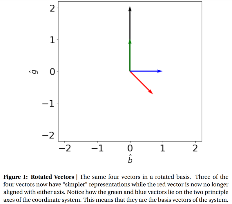
When written out:

As you can see from the above graph, and the written representations, three of our four new vectors are aligned with the axes!

While you might think this seems obvious, this is actually an example of something more subtle: this rotating transformation is our very first example of a change of basis!

Let’s break down how this change of basis happened. We started with some vectors in the original x, y basis (i.e. the standard cartesian basis) and applied some linear² operation (Yes! Rotations are linear operations) to transform the vectors into a “new” basis. The next question you might ask is: what do these new basis vectors look like? As it turns out, I hid the new basis vectors in Figure 1: \(\vec{b}\) and \(\vec{g}\) are the basis vectors for this new rotated basis (You can also check the axes in figure 2)! To further convince yourself that this is true, consider the following questions: How many copies of the green vector and how many copies of the blue vector are needed to build the blue vector? Only one blue vector (and no multiples of the green vector), therefore the representation of the blue vector in the new basis is \((1, 0)\). Similarly, how many multiples of the blue and green vectors are needed to build the black vector? We need 0 blue vectors, but 2 green vectors, therefore the representation of the black vector in the new basis is \((2, 0)\).

One key observation (which we will discuss further in the subsequent sections), is that when the basis vectors for the new rotated coordinate system are transformed from the standard cartesian coordinate system to the new rotated coordinate system, their representations in the rotated coordinate system are always aligned with individual axes and will have unit length. This means that their representations in the new coordinate system will be of the form \((1, 0, 0, …..)\) or \((0, 1, 0, 0, ….)\) or \((0, 0, 1, 0, ….)\) and so on. That is to say that they will be entirely zeros except for a single location where they have a one. (At the risk of spoiling a later punchline, the basis transformation matrix is the matrix which takes a matrix whose columns are the basis vectors in the standard basis and transforms them into the identity matrix.)

While this may not seem consequential, this observation is what ultimately allows us to build a change of basis matrix. That is, a matrix which takes any vector in the “standard” basis and returns the vector’s representation in the “new” basis.

A (More) General Change of Basis

In our previous example, we understood, somewhat intuitively, that when we rotated our coordinate system by 45 degrees, the resulting vectors would have a simpler representations. While it is easy enough to guess the resulting vectors when the rotation is a commonly used angle (i.e. 30, 45, 60, 90), it’s less obvious when the rotation is 10 degrees or 1 radian. Let’s try to find an exact mathematical way of representing any rotation matrix.

Suppose we want to rotate the basis vectors clockwise by \(\theta\) degrees. This means that instead of using our original basis vectors

we want to express every possible vector as a combination of the new basis vectors:

Visually, the new vectors are given by the blue vectors below:

The key question now is: how do we find the representation of any vector, \(\vec{z} = (x,y)\) with the new vectors? Put another way, we need to find how much of each of the new basis vectors are needed for \(\vec{z}\). Mathematically, we need to solve the following equation for a and b:

We can simplify the above expression if we combine the basis vectors, \(\hat{e_1}\) and \(\hat{e_2}\) into a single matrix. This results in the suggestive form:

Since we wanted to solve for a and b, we need to take the inverse of the “basis vector matrix”:

When you take the inverse of the above matrix (left as an exercise for the reader), you’ll find that this matrix is the standard rotation matrix used in linear algebra. It lets us take any vector \(\vec{z}\) and apply a rotation such that the resulting vector \((a, b)^T\) looks like it’s been rotated by an angle \(\theta\).

Now, you might have noticed that the only place where we used knowledge about the rotation was during the creation of the new basis vectors. You might be wondering, then, what would happen if we placed different basis vectors in the matrix, say ones that are neither mutually orthogonal nor unit-length. Well, it turns out that as long as the basis vectors are linearly independent, the inverse of that matrix give us a valid way to convert any vector between the standard basis and the second basis.

Orthonormality

When it comes to discussing bases, it turns out that not all basis vectors are created equal. As a general rule, orthonormal basis vectors are generally easier to work with. Orthonormality means that the basis vectors are all mutually orthogonal and that the vectors all have unit length.

One of the reasons that orthonormal bases are nice to work with is that taking the inverse of an orthonormal matrix is easy:

For real numbers:

$$A^{-1} = A^T$$

For complex numbers³:

$$A^{-1} = A^H$$

This is important because matrix inverses are often computationally expensive to compute⁴, however if we have an orthonormal basis (Hint, the Fourier basis) it makes finding the “change of basis matrix” much easier to calculate!

(The punchline) Fourier Transform as a change of basis:

Now that we’ve introduced all of the requisite material, we will now show that the Fourier transform is a change of basis. Let’s first consider a length N signal. The Fourier transform tells us that the length N signal can be decomposed into N sinusoids. Specifically, the sinusoids that we consider are of the form:

$$e^{i 2\pi k \frac{n}{N}}, k \in [0, N-1] \cap \mathbb{Z}$$

where k is our “frequency” index and n is our “time” index. As we are about to see, these N sinusoids form an orthonormal basis.

Because there’s a lot going on in this equation, let’s make things more concrete by considering the case where N = 18. Fig. 3 shows four of the eighteen possible sinusoids.

For those of you wondering what happened to the N/2 + 1 sines and N/2 + 1 cosines used in most traditional introductions of the Fourier transform (such as the one I gave in my last blog post), it turns out that these two representations are equivalent due to Euler’s formula

$$e^{i \phi } = \cos\left(\phi \right) + i \sin\left(\phi \right)$$

or written in a more mathematically suggestive form:

$$e^{i 2 \pi k \frac{n}{N}} = \cos\left(2 \pi k \frac{n}{N}\right) + i \sin\left(2 \pi k \frac{n}{N}\right)$$

It turns out that when we use the exponential formalism, that we are simultaneously finding the necessary cosines and sines together.

Next, we will show that these vectors are a valid basis for an N-dimensional space. As we will show, the N vectors that we have defined above are not only linearly independent (i.e. form a basis for an N-dimensional space), but are (with a proper scaling factor) orthonormal (i.e. form an especially “nice”/useful basis). To prove orthogonality, we need to show that the dot product (we will use \(\langle \cdot | \cdot \rangle\)to denote dot/inner product) between all vectors is zero when the two vectors are different (i.e. \(k_1 \neq k_2\)) and non-zero when the two vectors are the same (i.e. \(k_1 \eq k_2\)). This is from the definition of dotproduct: \( \vec{a}\cdot\vec{b}=|a||b|\cos(\theta) \) . Thus the dot product is zero when the angle between the vectors (\(\theta\)) is zero. Let’s start by proving that the inner product (dot product) between vectors with the same frequency is non-zero⁵:

Because orthonormality requires that all the vectors have unit length (not lengths = N), we need to divide all the vectors by \(\sqrt{N}\).

Proving that the inner product between any two different frequency vectors is 0 is a little bit more tricky:

The trick to solving this equation is to factor out n from the exponential.

Next, we need to recognize that this is a finite geometric sequence in n. With that in mind, we can therefore apply the equation for finite sums of geometric series⁶:

Applied to our situation:

For now let’s just focus on the numerator since the denominator will always be non-zero since k1 != k2. Looking at the numerator, we know \(k_1 - k_2\) will always be an integer. This means that \(e^{i2pi (k1-k2)}\) will always be equal to 1 (if this is not clear, see Euler’s formula above).

To recap, what we just proved is that these N sinusoids form an orthonormal basis for a N-dimensional vector space.

The next step is to project our length-N signal \(\vec{x}\) onto this Fourier basis (i.e. change to the Fourier basis). How do we convert our signal to the Fourier basis? As we derived previously, we simply collect all basis vectors into the columns of a matrix and then invert the matrix.

Expressed mathematically:

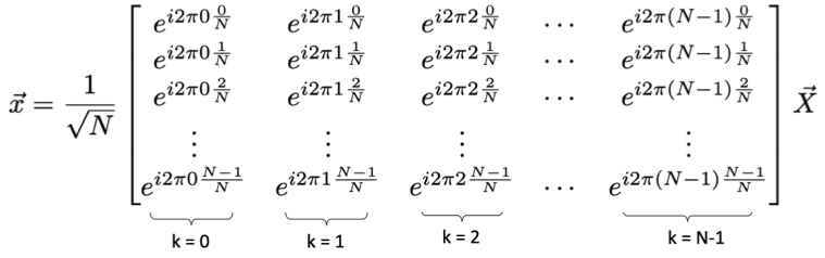
The above matrix can be confusing, so I find that it’s best to think of the matrix as a collection of columns where for each column corresponds to a different k. Furthermore, it’s worthwhile to remember that we already plotted what the columns should look like in fig 3.

When we invert the matrix, we can solve for \(\vec{x}\), which is the representation of our signal in the Fourier basis.

Now, it might seem intimidating to invert an arbitrarily-large NxN matrix, but we’re in luck. Because our matrix is orthonormal, it’s inverse is simply its conjugate transpose (Hermitian conjugate). This inverse matrix is known as the Fourier transform matrix:

$$\vec{X} = \mathfrak{F}\vec{x}$$

A note of warning here before we go further: This version of the Fourier transform matrix that I’ve introduced is the unitary version of the Fourier transform matrix. The only difference between it and the more commonly used Fourier transform matrix is the scalar factor of \(\frac{1}{\sqrt{N}}\) which doesn’t appear in the more traditional version⁷.

In the above inverse matrix, all of our columns shown in the first matrix have now been transposed into row vectors and have been conjugated (all imaginary parts now have a minus sign in front).

Most importantly, this equation here is exactly equal to the discrete Fourier transform.

If you’re wondering why it doesn’t look like the representation that you’re most likely familiar with, the answer is that in most representations of the Fourier transform, the notation is compressed. Rather than write out the full matrix equation, a simpler equation for the kth frequency term is given instead. Because we are multiplying a matrix by a vector, the equation for \(X[k]\) is the dot (inner) product of the input vector \(x[n]\) with the k th row of the matrix (i.e. \(\mathfrak{F}[k,i]\) for I = 0 to N-1). When we do this to our above equation, this gives the familiar Fourier transform equation (ignoring the scalar factor):

$$X[k] = \sum_{n=0}^{N-1}x[n]e^{-2\pi k \frac{n}{N}}$$

Tada! That’s it! We’ve now come full circle. Let’s recap our adventure: we started by showing how change of bases might be useful, and then figured out how to derive an arbitrary change of basis matrix. Next, we considered a very particular orthogonal basis, the “Fourier” basis and lastly, we showed that when a signal is transformed to the “Fourier” basis, its new representation is the “frequency domain” representation. This shows conclusively that the Fourier transform is really just a linear algebraic change of basis.

Outro

You next question might be “so what? Who cares that the discrete Fourier transform is a change of basis?” The answer that I propose is that you do! Now that we’ve demonstrated the connection between Fourier analysis and linear algebra, we can use the powerful “machinery” of linear algebra whenever thinking about Fourier analysis!

For example, I could never figure out why after all these summations (or integrations), that the inverse Fourier transform would perfectly cancel out the Fourier transform. But when these transformations are thought of as conversions from one base and then back again, it becomes almost intuitive that they should cancel eachother out.

As a more advanced example, I also like the intutition that this approach gives Parseval’s theorem. Which states that the time domain and frequency domain representations contain equal amounts of power. Because the Fourier transform matrix is unitary (orthonormal), the “length” of the input vector is not changed when converting from the time to frequency bases. Since length-squared is proportional to power for signals, the fact that the lengths are the same mean that the power contained by the representations is also the same!

Furthermore, the results that we’ve derived here are applicable to the various other versions of the Fourier transform (e.g. continuous time, 2D, 3D, etc.). Unfortunately, those derivations are up to you. While the reduction of the Fourier transform to a matrix multiplication is only valid for discrete Fourier transform, many of the other statements still hold. Most importantly, we can think of any of the other Fourier transforms as projections of time-domain signals onto the Fourier basis with the appropriate frequencies.